Portfolio 3 IA

Posted Nov 6, 2023 Updated Dec 12, 2023

By Danilo Carvalho Antunes 15 min read

Intruduction

Constraint Satisfaction Problems (CSPs) are a foundational concept in computational theory and artificial intelligence, where the task is to find a combination of values that satisfies a set of constraints over given variables. In exploring CSPs, we encounter different strategies for representing the problem atomic representation treats each state as an indivisible unit, while factored representation breaks down states into a more granular view using variables or factors. The types of constraints unary, binary, and n-ary determine the interactions between these variables and play a crucial role in defining the complexity of the problem.

To navigate through the potential solutions of a CSP, we rely on various levels of consistency checks, such as node consistency, arc consistency, and global consistency, each offering a measure to evaluate the feasibility of solutions. The choice of algorithm to resolve these problems can greatly impact the effectiveness and efficiency of the solution, with backtracking, forward checking, and constraint propagation (like AC-3) being among the most prevalent methods.

In this text, we will explore these concepts, examining how they contribute to the structure and solvability of CSPs, and how they can be applied to problems represented in graph structures, enhancing our understanding and approach to solving these intricate computational puzzles.

Constraint Satisfaction Problem (CSP)

Constraint Satisfaction Problems (CSPs) are a category of computational problems that are centered around finding states that satisfy a collection of constraints. Each CSP consists of three main components:

Variables: These are the elements that need to be assigned values from their possible domains. They can be anything from colors in a coloring problem, digits in a sudoku, to timeslots in a scheduling task.
Domains: For each variable, there is a corresponding domain which is the set of all possible values that the variable can take. For example, in a sudoku puzzle, the domain for each cell (variable) is the numbers 1 through 9.
Constraints: These are rules that must be followed for a solution to be considered valid. Constraints can be binary, involving two variables (such as “Variable A must be different from Variable B”), or they can be more complex, involving three or more variables. The constraints define the relationships between the variables and restrict the values the variables can simultaneously take.

Atomic representation and Factored representation

In the realm of Constraint Satisfaction Problems (CSPs), two primary methodologies for state representation are atomic representation and factored representation.

Atomic representation regards each state as an indivisible “black box” with no internal structure. This approach to CSPs is straightforward, as it does not acknowledge the complexities within a state, treating each state as a whole unit. It’s a like to seeing a picture as a single entity without recognizing the individual pixels that compose it.

Factored representation, on the other hand, deconstructs states into variables or “factors”. Each factor is endowed with its distinct set of possible values, which enables a detailed inspection of the state’s condition. Imagine a puzzle where each piece represents a factor; only by fitting these pieces together in the correct way can the overall picture be revealed. This approach show a more expressive portrayal of states and can enhance the efficiency of CSP resolution. By breaking down the problem into smaller, manageable sub-problems, factored representation often facilitates the discovery of a solution through the individual resolution of these components.

In essence, while atomic representation simplifies the complexity of CSPs by treating each state as a single, unbreakable element, factored representation embraces this complexity by splitting states into multiple, interrelated factors. Each method has its merits and is suitable for different types of CSPs, depending on the level of detail required and the nature of the problem at hand.

Types of Conditions

In the study of Constraint Satisfaction Problems (CSPs), there are several types of conditions or constraints that can be imposed on variables:

Unary Constraints: These involve only a single variable and restrict the value that the variable can take. An example of a unary constraint could be a rule stating that a certain task must be done by a specific team member.
Binary Constraints: These involve pairs of variables and specify a relation between their values. For instance, in a scheduling problem, a binary constraint might require that two tasks cannot be scheduled at the same time or that one task must be completed before another can begin.
N-ary Constraints: These involve ‘n’ number of variables, where ‘n’ can be any integer greater than two. N-ary constraints deal with relations among three or more variables. For example, a constraint in a resource allocation problem may state that the combined effort of three different workers is needed to complete a job.

Node Consistency

In the context of Constraint Satisfaction Problems (CSPs), consistency is a key concept used to assess the solvability of the problem. It is evaluated at different levels:

Node Consistency: Thi# Intruductions level checks whether each individual variable in the CSP can satisfy its own constraints. Essentially, node consistency ensures that every value in a variable’s domain meets the variable’s unary constraints.
Arc Consistency: This involves looking at each pair of variables and checking if there is some way to assign values to both such that their binary constraints are satisfied. For a CSP to be arc-consistent, every value in a variable’s domain must be consistent with every possible value of each neighboring variable’s domain.
Path Consistency: This extends the concept of arc consistency to sequences of variables, ensuring that not just pairs, but triples of variables can be assigned values without violating their binary constraints.
k-Consistency: This generalizes the notion of arc consistency for a set of k variables, where k is any positive integer. A CSP is k-consistent if for any set of k - 1 variables and for any consistent assignment to these variables, a consistent value can be assigned to a kth variable.
Global Consistency: This is the most stringent level, which checks whether the entire set of variables in the CSP can be assigned values simultaneously without violating any constraints.

Algorithms

The selection of an algorithm to solve a Constraint Satisfaction Problem (CSP) can greatly depend on the nature of the problem at hand. Here are three of the most commonly used algorithms:

Constraint Propagation (AC-3 Algorithm): Utilizing the concept of arc consistency, this algorithm reduces the domain size of each variable by repeatedly checking all the constraints and eliminating values that cannot possibly participate in a complete solution. It ensures that for each variable, every value in its domain has a consistent value in the domain of adjacent variables. AC-3 can be used in conjunction with backtracking, where arc consistency is maintained at each step of the search, significantly enhancing the efficiency of the search process.
Backtracking: This depth-first search method attempts to solve the problem by sequentially assigning values to variables. If at any point the current assignment does not lead to a solution, the algorithm “backtracks” to the previous step and tries a different value. This recursive algorithm can be optimized with variable selection heuristics (such as the minimum remaining value heuristic) and value ordering heuristics (like least constraining value heuristic), which help to reduce the number of backtracking occurrences.
Forward Checking: As values are assigned to variables, forward checking immediately checks the constraints that involve the variable that just had a value assigned. This helps to look ahead and eliminate from other variables’ domains any values that would result in a violation of constraints, thereby reducing the possible search space. If at any point the domain of a variable becomes empty, the algorithm backtracks, ensuring that decisions do not lead to a dead end.

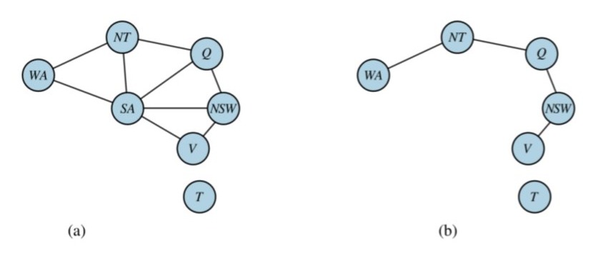
Structure of Problems for Graphs

To solve tree CSPs we do the following:

We choose a variable as the root;

We order the tree so that each variable appears after its parent in the tree (topological classification);

Topological classidication

Cutting conditioning

Cutting conditioning

Tree decomposition

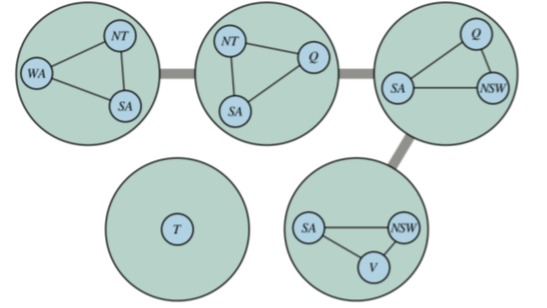
Tree decomposition

Each variable in the original problem appears in at least one of the nodes in the tree.

If two variables are connected by a constraint in the original problem, they must appear together (along with the constraint) in at least one of the tree nodes.

If a variable appears in two nodes in the tree, it must appear in all nodes along the path connecting those nodes.

Contributions

The study of Constraint Satisfaction Problems (CSPs) is rich with varied contributions that expand beyond the basic concepts previously discussed. To delve deeper into this field, we can explore several other important aspects:

Heuristics and Optimization in CSPs: Beyond the fundamental representations and algorithms, there are numerous heuristics designed to optimize the search process in CSPs. These include techniques like least constraining value, which chooses the next value to assign by selecting the one that will leave the maximum flexibility for subsequent variable assignments.
Dynamic Variable Ordering: The efficiency of solving a CSP can be further enhanced by dynamically choosing the order of variables as the search progresses, adapting the strategy based on the state of the problem at each step. This contrasts with static variable ordering and allows for more flexibility and efficiency in the search process.
Decomposition and Hybrid Representations: CSPs can also be tackled by decomposing them into smaller, more manageable sub-problems. This can involve a hybrid approach that combines atomic and factored representations, which can be particularly effective when dealing with complex constraints that are neither purely atomic nor easily factorable.
Graph-Based Representations and Analysis: When representing CSPs as graphs, one can employ various graph algorithms and properties, such as finding strongly connected components or utilizing coloring algorithms, to simplify the problem or to identify the most constrained parts of the problem more quickly.

Each of these contributions has expanded the toolbox available for tackling CSPs, allowing for the design of more efficient and effective algorithms and for the CSP framework to be applied to increasingly complex and diverse problems.

Optimization in CSPs

In applications such as industrial scheduling, some solutions are better than others. In other cases, the assignment of different values to the same variable incurs different costs. The task in such problems is to find optimal solutions, where optimality is defined in terms of some application-specific functions. We call these problems Constraint Satisfaction Optimization Problems (CSOP) to distinguish them from the standard CSP.

Finding optimal solutions basically involves comparing all the solutions in a CSOP. Therefore, techniques for finding all solutions are more relevant to CSOP solving than techniques for finding single solutions.

Variable ordering techniques which aim at minimizing backtracking (the minimal width ordering) and minimizing the number of backtracks (the minimal bandwidth ordering) are more useful for finding single solutions than all solutions. On the other hand, the fail first principle (FFP) in variable ordering is useful for finding all solutions as well as single solutions, because it aims at detecting futility as soon as possible so as to prune off more of the search space.

Zebra Puzzle

Implementation in Python code of algorithms and/or problems not discussed in class

Tools From Wikipedia, the free encyclopedia The Zebra Puzzle is a well-known logic puzzle. Many versions of the puzzle exist, including a version published in Life International magazine on December 17, 1962. The March 25, 1963, issue of Life contained the solution and the names of several hundred successful solvers from around the world.

The puzzle is often called Einstein’s Puzzle or Einstein’s Riddle because it is said to have been invented by Albert Einstein as a boy; it is also sometimes attributed to Lewis Carroll. However, there is no evidence for either person’s authorship, and the Life International version of the puzzle mentions brands of cigarettes that did not exist during Carroll’s lifetime or Einstein’s boyhood.

The Zebra puzzle has been used as a benchmark in the evaluation of computer algorithms for solving constraint satisfaction problems.

Description The following version of the puzzle appeared in Life International in 1962:

There are five houses.
The Englishman lives in the red house.
The Spaniard owns the dog.
Coffee is drunk in the green house.
The Ukrainian drinks tea.
The green house is immediately to the right of the ivory house.
The Old Gold smoker owns snails.
Kools are smoked in the yellow house.
Milk is drunk in the middle house.
The Norwegian lives in the first house.
The man who smokes Chesterfields lives in the house next to the man with the fox.
Kools are smoked in the house next to the house where the horse is kept.
The Lucky Strike smoker drinks orange juice.
The Japanese smokes Parliaments.
The Norwegian lives next to the blue house.

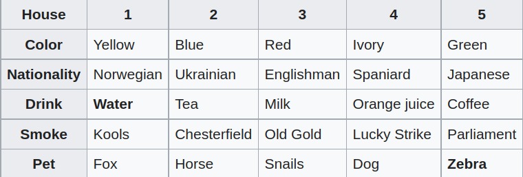
Now, who drinks water? Who owns the zebra?

In the interest of clarity, it must be added that each of the five houses is painted a different color, and their inhabitants are of different national extractions, own different pets, drink different beverages and smoke different brands of American cigarets. One other thing: in statement 6, right means your right.

— Life International, December 17, 1962

The answer of this puzzle is determined by checking all the constraints and building the solution step by step. More details about the problem and the solution can be found in the Wikipedia reference. Let’s see how we can code the solution in Go.

Solution for the Zebra Puzzle

Code

  
package zebra

// CSP is a structure that models a
// simple constraint satisfaction problem
type CSP struct {
	v, d []uint8
	c    []constrainter
}

// SolvePuzzle function solves the zebra puzzle
func SolvePuzzle() Solution {
	csp := CSP{
		v: make([]uint8, 30),
		d: []uint8{1, 2, 3, 4, 5},
		c: []constrainter{
			constraint(partialSolution),
			togetherWithConstraint{a: englishman, b: red},
			togetherWithConstraint{a: green, b: coffee},
			togetherWithConstraint{a: spaniard, b: dog},
			togetherWithConstraint{a: ukrainian, b: tea},
			toTheRightOfConstraint{a: green, b: ivory},
			togetherWithConstraint{a: oldGold, b: snails},
			togetherWithConstraint{a: kools, b: yellow},
			togetherWithConstraint{a: milk, b: house3},
			togetherWithConstraint{a: norwegian, b: house1},
			nextToConstraint{a: chesterfields, b: fox},
			nextToConstraint{a: kools, b: horse},
			togetherWithConstraint{a: luckyStrike, b: orangeJuice},
			togetherWithConstraint{a: japanese, b: parliaments},
			nextToConstraint{a: norwegian, b: blue},
		},
	}
	recursiveBacktracking(&csp.v, &csp)
	return Solution{OwnsZebra: ownerOf(zebra, csp.v...), DrinksWater: ownerOf(water, csp.v...)}
}

func recursiveBacktracking(assignment *[]uint8, csp *CSP) bool {
	if complete(csp.v) {
		return true
	}
	idx := selectUnassigned(&csp.v, assignment, *csp)
domainValueLoop:
	for _, d := range csp.d {
		csp.v[idx] = d
		for _, c := range csp.c {
			switch {
			case !c.forApplicability()(csp.v...):
				continue
			case !c.forSatisfaction()(csp.v...):
				csp.v[idx] = 0
				continue domainValueLoop
			default:
			}
		}
		outcome := recursiveBacktracking(assignment, csp)
		if !outcome {
			csp.v[idx] = 0
			continue domainValueLoop
		}
		return true
	}
	return false
}

func selectUnassigned(variables, assignment *[]uint8, csp CSP) uint8 {
	for _, c := range csp.c {
		indexer := func([]uint8) (uint8, bool) { return 0, false }
		switch constr := c.(type) {
		case togetherWithConstraint:
			indexer = constr.forMissingIndex
		case nextToConstraint:
			indexer = constr.forMissingIndex
		}
		idx, ok := indexer(*variables)
		if !ok || (*variables)[idx] != 0 {
			continue
		}
		return uint8(idx)
	}
	for i, v := range *assignment {
		if v != 0 {
			continue
		}
		return uint8(i)
	}
	return 0
}

func complete(assignment []uint8) bool {
	for _, v := range assignment {
		if v != 0 {
			continue
		}
		return false
	}
	return true
}

// Solution type describes the solution of the zebra puzzle
type Solution struct {
	DrinksWater string
	OwnsZebra   string
}

Solving the CSP in Go A typical solution to a CSP is a recursive backtracking algorithm:

Check if the all the variables inside the CSP are assigned, if yes return success, if not continue.
Select an unassigned variable x.
For each domain value, assign the value to the unassigned variable x.
For each constraint check if it can be applied, if yes continue, if not skip to the next constraint.
If the constraint can be applied, check if the current set of variables satisfy the constraint, if yes continue to step 6, if not unassign the variable x and skip to the next domain value (step 3).
Keep the assigned variable x and call this algorithm recursively.
If all domain values are looped without satisfying the constraint set a failure is returned and we backtrack one step down.

Conclusion

In conclusion, Constraint Satisfaction Problems (CSPs) offer a comprehensive framework for solving complex problems through variable and constraint management. This text covered different CSP representations, such as atomic and factored, along with constraint types (unary, binary, n-ary) that dictate problem complexity. Consistency levels from node to global are critical for evaluating solution viability, with algorithms like backtracking, forward checking, and constraint propagation serving as navigational tools through solution spaces, often utilizing graph structures for enhanced clarity and efficiency. CSPs integrate multiple disciplines to evolve problem-solving approaches, promising continued advancements in tackling increasingly complex computational challenges.

References

http://cse.unl.edu/~choueiry/Documents/TsangTextbook/ch10.pdf
https://en.wikipedia.org/wiki/Zebra_Puzzle
https://medium.com/@nikiforos_frees/solving-the-zebra-puzzle-using-go-7d3a4084e057#:~:text=As%20the%20Wikipedia%20page%20mentions,which%20all%20constraints%20are%20satisfied.
https://github.com/mcaci/zebra-puzzle-example

studies, ai, portfolio3

ai studies

This post is licensed under CC BY 4.0 by the author.